
Finding True Value in Fantasy Baseball — A Common Currency (3/6)
Part 3: Z-Scores — A Common Currency
TRP — True Relative Price: True Value. Market Pricing. No Noise.
Part 1 established the problem. Part 2 established the True Replacement Player — a composite archetype representing the baseline at each position. Now we can measure how far above (or below) that baseline each rostered player sits.
But there’s a problem. A catcher who’s +10 HR above replacement and +5 SB above replacement and +.350 OBP above replacement — what’s his total value?
You can’t just add those numbers. They’re measured in different units, with different scales, with different distributions. Ten home runs and five stolen bases and .350 OBP don’t combine into 15.350 anything.
This is the category problem. And Z-scores are the solution.
The Category Problem, Revisited
Fantasy baseball forces you to optimize across multiple categories simultaneously. In a standard 5x5 league, you’re balancing:
Hitting: R, HR, RBI, SB, AVG (or OBP) Pitching: W, SV, ERA, WHIP, K
Each category has its own scale:
- HR range from 0 to ~50
- SB range from 0 to ~70
- OBP ranges from ~.280 to ~.400
And each category has its own distribution. The difference between 30 HR and 35 HR might be huge (moving from 50th percentile to 80th), while the difference between 5 SB and 10 SB might be trivial (moving from 20th to 25th percentile) depending on your league’s composition.
Raw stats can’t capture this. You need a transformation that puts every category on the same scale — one where the units represent relative standing, not absolute production.
What Z-Scores Actually Measure
A Z-score answers a simple question: How many standard deviations is this value from the reference point?
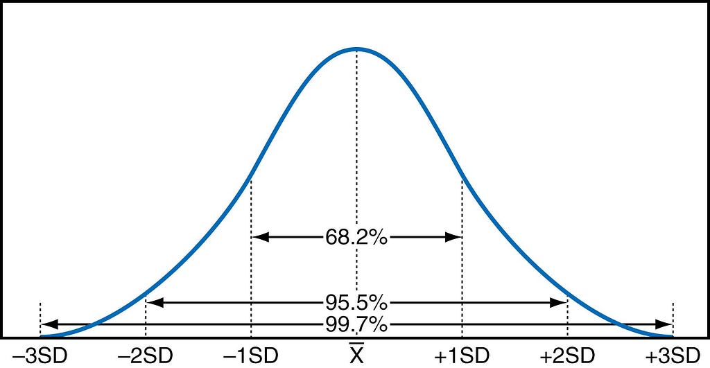
If you remember the bell curve from statistics class, there’s a rule called the 68–95–99.7 rule (or empirical rule): in a normal distribution, about 68% of values fall within 1 standard deviation of the mean, 95% within 2 standard deviations, and 99.7% within 3.
Flip that around and it tells you how rare a player is:
- Z = +1.0 means the player is better than ~84% of the pool (the 50% below average plus half of the 68% within 1 SD)
- Z = +2.0 means the player is better than ~97.5% of the pool
- Z = +3.0 means the player is in the top 0.15% — a true outlier
This is what makes Z-scores powerful: they translate raw production into percentile rarity.
The formula:
Z = (Player Stat − Reference Stat) / Standard Deviation
In TRP, the reference point is the True Replacement Player archetype. So the Z-score tells you: How many standard deviations above replacement is this player in this category?
A Z-score of +1.0 means the player is one standard deviation above the replacement baseline. A Z-score of 0 means the player is exactly at replacement level. A Z-score of -0.5 means the player is half a standard deviation below replacement — he’s actively hurting you.
The beauty: once every category is expressed in standard deviations, you can add them. A player with +1.5 in HR and +0.8 in SB and +1.2 in OBP has a total Z of +3.5. That’s a meaningful composite value.
A Concrete Example
Let’s walk through a shortstop valuation using real 2026 projections.
Step 1: Establish the replacement tier.
In a 12-team league with one SS slot, the top 12 shortstops are rostered. Here we provide the seed (initial) sort by wRC+ because it’s sabermetrics best attempt at reducing all offensive production to a single metric.
Sorting by wRC+:
| Rank | Player | wRC+ |
|---|---|---|
| 1 | Fernando Tatis Jr. | 142.0 |
| 2 | Corey Seager | 135.3 |
| 3 | Gunnar Henderson | 135.0 |
| ... | ... | ... |
| 8 | Geraldo Perdomo | 119.4 |
| ... | ... | ... |
| 11 | Jorge Polanco | 116.1 |
| 12 | Carlos Correa | 115.2 |
| 13 | Trea Turner | 113.1 |
| 14 | Zach Neto | 112.8 |
| 15 | Kevin McGonigle | 111.1 |
| 16 | Xander Bogaerts | 111.0 |
Carlos Correa is the last rostered SS at 115.2 wRC+. A 3% band captures everyone down to ~112.2 — that’s only Trea Turner (113.1) and Zach Neto (112.8). Two players.
TRP enforces a minimum tier size of 3 players to avoid fragile baselines. When the initial band captures fewer than 3, we expand by 1% increments until we hit the minimum. A 4% band (down to ~111.1) captures Turner, Neto, and McGonigle — three players, minimum met.
Step 2: Compute the True Replacement SS archetype.
Average the projected stats across the replacement tier:
| Stat | Turner | Neto | McGonigle | Replacement SS |
|---|---|---|---|---|
| R | 85.4 | 83.1 | 23.8* | 64.1 |
| HR | 17.9 | 26.0 | 5.1* | 16.3 |
| RBI | 64.9 | 69.7 | 21.9* | 52.2 |
| SB | 26.2 | 26.9 | 3.8* | 19.0 |
| OBP | .332 | .320 | .340 | .331 |
| SLG | .441 | .456 | .410 | .436 |
*McGonigle’s counting stats are lower due to projected playing time (50 games).
A Note on Rate Stats and Playing Time
Some valuation systems weight rate stats (AVG, OBP, ERA, WHIP) by playing time — multiplying a player’s OBP Z-score by his projected plate appearances, for instance. The logic: a .350 OBP in 600 PA is more valuable than a .350 OBP in 400 PA.
TRP doesn’t do this, for two reasons:
1. Counting stats already reflect playing time.
A player projected for 400 PA is already getting fewer R, HR, RBI, and SB than a 600 PA player. His counting stat Z-scores are lower as a result. Weighting his rate stats by PA penalizes him twice for the same limitation.
2. The roster slot doesn’t sit empty.
If your starter only plays 120 games, someone plays the other 42. To accurately weight rate stats, you’d need to composite your starter’s rates with the replacement player’s rates for the games missed — a .350 OBP for 120 games plus a .310 OBP for 42 games, weighted appropriately.
That’s doable, but it adds complexity without clearly improving accuracy. And it raises questions: which replacement player? What if you stream the slot? What if injuries create a three-way timeshare?
TRP keeps it simple. Rate stats are compared directly. Counting stats handle the playing time adjustment. The result is a cleaner system that’s easier to reason about and validate.
Back to our example. For the replacement archetype, we’ll use the full-season projected rate stats (OBP, SLG) which remain comparable regardless of playing time.
Step 3: Compute standard deviations across the rostered tier (top 12 SS).
| Stat | σ (Standard Deviation) |
|---|---|
| OBP | .014 |
| SLG | .032 |
Step 4: Calculate Z-scores for Geraldo Perdomo.
Let’s take a deeper look at Perdomo’s 2026 projections: .365 OBP, .412 SLG
| Category | Perdomo | Replacement | Perdomo − Repl | σ | Z-Score |
|---|---|---|---|---|---|
| OBP | .365 | .331 | +.034 | .014 | +2.43 |
| SLG | .412 | .436 | -.024 | .032 | -0.75 |
Even in just these two categories, you can see Perdomo’s split personality: elite OBP (+2.43 Z, better than ~99% of the pool), below replacement in SLG (-0.75 Z).
Extend this across all six hitting categories and the pattern holds. Perdomo’s value is extremely lopsided — he’s an on-base machine with minimal power. In a format where each category counts independently, his elite OBP can’t fully compensate for his liabilities in HR, RBI, and SLG.
This is exactly why Z-scores matter. Looking at raw projections, Perdomo seems fine — he’s the 8th-ranked SS by wRC+. But wRC+ weights everything into one number. Fantasy leagues score categories separately. A player who’s +3 in one category and -1 in three others isn’t neutral; he’s a specialist whose value depends entirely on your team’s category needs.
Total Z vs. Category Z: Draft Strategy
This brings up an important point: total Z isn’t the only number that matters.
When drafting, you’re building a portfolio across categories. If your first seven picks were power-heavy (strong HR, RBI, SLG) but weak in OBP, a player like Perdomo becomes strategically valuable — not despite his lopsided profile, but because of it.
His +2.43 OBP Z-score fills a gap. You can quantify exactly how much he improves your team’s OBP standing relative to the league. That’s the power of category-level Z-scores: they let you draft for balance, not just total value.
Total Z tells you overall value. Category Z tells you where the value comes from — and whether it’s value your team actually needs.
A well-constructed roster isn’t necessarily the one with the highest total Z (but good luck making the playoffs if your total Z is low). It’s the one with competitive Z-scores across all categories — no glaring holes for opponents to exploit.
Why Standard Deviation Matters
The denominator — standard deviation — is doing critical work here.
Standard deviation measures how spread out the values are. A category with high variance (lots of difference between the best and worst) will have a large standard deviation. A category with low variance (everyone’s clustered together) will have a small one.
This matters because a 5-HR improvement means different things in different contexts:
- If the standard deviation is 10 HR, then +5 HR is only +0.5 Z — half a standard deviation, modest improvement.
- If the standard deviation is 3 HR, then +5 HR is +1.67 Z — nearly two standard deviations, a major leap.
The Z-score automatically adjusts for this. Categories where production is tightly clustered get amplified; categories where production is spread out get compressed. The result is a fair comparison.
Computing Standard Deviation: Which Pool?
There’s a subtle but important choice: which players do you include when computing standard deviation?
Option 1: All players at the position. This includes replacement-level scrubs, inflating variance and compressing Z-scores for everyone.
Option 2: Only the rostered tier. This captures the variance among players who actually matter — the ones you’re deciding between.
TRP uses Option 2. The standard deviation is computed across the rostered tier only (e.g., the top 12 shortstops in a 12-team league). This ensures the Z-scores reflect meaningful distinctions among draftable players, not noise from the waiver wire.
Handling Inverted Categories
Not all stats work the same direction. For hitting categories, higher is better — more HR, more SB, higher OBP. But for pitching ratios, lower is better — lower ERA, lower WHIP.
For inverted categories, flip the formula:
Z = (Reference Stat − Player Stat) / Standard Deviation
This ensures a pitcher with a 3.00 ERA (good) gets a positive Z-score when the replacement ERA is 4.20 (bad), rather than a negative one.
TRP applies this inversion to ERA and WHIP. All other categories use the standard formula.
Role-Based Zeroing
One more nuance: not every player contributes to every category.
Starting pitchers don’t earn saves. Relief pitchers don’t earn quality starts. For this reason SPs and RPs are not combined for valuations; we have hitters, starting pitchers, and relief pitchers as distinct position types. If you kept all pitchers together and then applied the standard Z-score formula, a starter would get a massive negative Z in saves (0 saves vs. replacement), which makes no sense — he’s not failing to save games, he’s just not a closer.
TRP handles this with role-based zeroing:
- SP: Z_SVHD = 0 (saves/holds not applicable)
- RP: Z_QS = 0 (quality starts not applicable)
The player isn’t penalized for categories that don’t apply to their role.
From Category Z to Total Z
Once you’ve computed Z-scores for each category, sum them:
Hitters: Z_total = Z_R + Z_HR + Z_RBI + Z_SB + Z_OBP + Z_SLG
Pitchers: Z_total = Z_IP + Z_QS or Z_SVHD + Z_K9 + Z_ERA + Z_WHIP
But there’s one more step: normalization to replacement level, a.k.a. replacement baseline shift (z̄_RLP).
The Z-scores we’ve calculated so far are relative to the replacement tier’s raw stats. But we want replacement-level players to have a Z-score of zero — that’s the baseline. If the replacement tier’s average SB Z-score comes out to -0.5, we need to shift everyone’s SB Z-score up by +0.5 so that replacement level equals zero.
This normalization ensures that:
- Replacement-level players have total Z ≈ 0
- Positive Z means above replacement
- Negative Z means below replacement
Iteration Process (Worked Example)
The initial sort by wRC+ is only a seed. It gives us a first guess at who’s rostered and who’s replacement-level. But wRC+ and category value (total Z) don’t always agree.
A player can be “good” in real baseball (high wRC+) while being mediocre in fantasy if they’re empty in key categories (like SB), or extremely lopsided (like OBP-only).
TRP fixes this using iteration: we keep re-defining rostered and replacement tiers based on total Z until the rostered tier stops changing.
The Loop (What TRP Does Each Pass)
Given:
- A roster size N at the position (here: 12 SS)
- A minimum replacement tier size K (here: 3 SS)
Each iteration:
- Identify rostered tier (top N players for this position).
- Compute rostered-tier distribution for each category: Mean (μ) and Standard deviation (σ).
- Compute raw category Z-scores for everyone using the rostered tier: z_raw = (stat − μ) / σ
- Define the replacement tier (next K players after the rostered tier).
- Compute the replacement-tier average raw Z using the standard deviation from the rostered-tier for each category: z̄_RLP (one value per category).
- Normalize so replacement level equals zero in every category: z_norm = z_raw − z̄_RLP
- Sum categories: Total Z = Σ z_norm (across R, HR, RBI, SB, OBP, SLG)
- Re-rank by Total Z, update tiers, repeat until rostered tier membership stops changing.
SORT 1: Initial wRC+ Rankings (Seed Pass)
| wRC+ Rank | Player | wRC+ |
|---|---|---|
| 1 | Fernando Tatis Jr. | 142.0 |
| 2 | Corey Seager | 135.3 |
| 3 | Gunnar Henderson | 135.0 |
| 4 | Bobby Witt Jr. | 132.6 |
| 5 | Francisco Lindor | 122.9 |
| 6 | Bo Bichette | 121.0 |
| 7 | Geraldo Perdomo | 119.4 |
| 8 | Jacob Wilson | 118.8 |
| 9 | Elly De La Cruz | 117.1 |
| 10 | Jorge Polanco | 116.1 |
| 11 | Carlos Correa | 115.2 |
| 12 | Trea Turner | 113.1 |
| 13 | Zach Neto | 112.8 |
| 14 | Kevin McGonigle | 111.1 |
| 15 | Xander Bogaerts | 111.0 |
| 16 | Jeremy Peña | 110.4 |
| 17 | Willy Adames | 108.2 |
| 18 | Nico Hoerner | 107.2 |
| 19 | CJ Abrams | 105.9 |
| ... | ... | ... |
Seed rostered tier (N=12): ranks 1–12 Seed replacement tier (min K=3): Neto, McGonigle, Bogaerts
ITERATION 1: Calculate Raw Z, Then Normalize to Replacement
Step 1: Rostered-tier distribution (μ and σ)
Rostered Tier Means: R=78.5, HR=21.0, RBI=70.9, SB=16.7, OBP=.346, SLG=.462
Rostered Tier SDs: R=15.1, HR=6.2, RBI=11.3, SB=12.5, OBP=.012, SLG=.031
Step 2: Replacement Tier Raw Z-Scores (before normalization)
| Player | zR | zHR | zRBI | zSB | zOBP | zSLG | Total |
|---|---|---|---|---|---|---|---|
| Zach Neto | 0.30 | 0.81 | -0.11 | 0.82 | -2.19 | -0.18 | -0.54 |
| Kevin McGonigle | -3.63 | -2.58 | -4.35 | -1.03 | -0.51 | -1.64 | -13.75 |
| Xander Bogaerts | -1.39 | -1.33 | -1.25 | -0.24 | -1.02 | -1.74 | -6.96 |
| RLP Average (z̄_RLP) | -1.57 | -1.03 | -1.90 | -0.15 | -1.24 | -1.19 | -7.09 |
Right now replacement averages -7.09 Total Z, but replacement level should be 0 by definition.
Step 3: Baseline shift (normalize to replacement)
Normalization: z_norm = z_raw − z̄_RLP
| Category | z̄_RLP | Shift = −z̄_RLP |
|---|---|---|
| R | -1.57 | +1.57 |
| HR | -1.03 | +1.03 |
| RBI | -1.90 | +1.90 |
| SB | -0.15 | +0.15 |
| OBP | -1.24 | +1.24 |
| SLG | -1.19 | +1.19 |
Sanity check: after applying these shifts, the replacement tier average in each category becomes 0.00.
Worked Example: Zach Neto (Raw → Normalized, With Stats)
Neto’s projection line: R=83.1, HR=26.0, RBI=69.7, SB=26.9, OBP=.320, SLG=.456
| Cat | Neto stat | μ | σ | z_raw | Shift | z_norm |
|---|---|---|---|---|---|---|
| R | 83.1 | 78.5 | 15.1 | 0.30 | +1.57 | 1.87 |
| HR | 26.0 | 21.0 | 6.2 | 0.81 | +1.03 | 1.84 |
| RBI | 69.7 | 70.9 | 11.3 | -0.11 | +1.90 | 1.79 |
| SB | 26.9 | 16.7 | 12.5 | 0.82 | +0.15 | 0.97 |
| OBP | .320 | .346 | .012 | -2.19 | +1.24 | -0.95 |
| SLG | .456 | .462 | .031 | -0.18 | +1.19 | 1.01 |
Total Z (raw) = -0.54
Total Z (normalized) = 1.87 + 1.84 + 1.79 + 0.97 – 0.95 + 1.01 = 6.54
That’s the core idea:
- Raw Z measures you relative to the rostered-tier average
- Normalized Z measures you relative to the replacement baseline (true “0”)
ITERATION 1 Results: Normalized Z Rankings
| Rank | Player | zR | zHR | zRBI | zSB | zOBP | zSLG | Total Z |
|---|---|---|---|---|---|---|---|---|
| 1 | Bobby Witt Jr. | 2.81 | 1.91 | 3.27 | 1.32 | 1.48 | 2.76 | 13.56 |
| 2 | Fernando Tatis Jr. | 2.82 | 2.54 | 2.53 | 0.71 | 2.41 | 2.50 | 13.52 |
| 3 | Gunnar Henderson | 2.26 | 1.93 | 3.36 | 0.53 | 2.07 | 2.03 | 12.18 |
| 4 | Elly De La Cruz | 1.86 | 1.41 | 2.88 | 1.82 | 0.90 | 1.33 | 10.20 |
| 5 | Francisco Lindor | 2.60 | 1.88 | 2.12 | 0.66 | 0.48 | 0.88 | 8.61 |
| 6 | Corey Seager | 1.06 | 1.67 | 2.17 | -0.98 | 2.24 | 2.31 | 8.47 |
| 7 | Zach Neto | 1.87 | 1.85 | 1.80 | 0.97 | -0.95 | 1.01 | 6.54 |
| 8 | Trea Turner | 2.03 | 0.53 | 1.37 | 0.91 | 0.06 | 0.53 | 5.43 |
| 9 | Bo Bichette | 1.36 | 0.47 | 1.86 | -0.71 | 0.81 | 0.98 | 4.76 |
| 10 | Geraldo Perdomo | 1.50 | -0.38 | 0.46 | 0.30 | 2.83 | -0.39 | 4.31 |
| 11 | Willy Adames | 1.52 | 1.49 | 2.12 | -0.31 | -0.87 | -0.20 | 3.74 |
| 12 | CJ Abrams | 1.55 | 0.74 | 1.28 | 1.08 | -1.37 | 0.15 | 3.43 |
| 13 | Jeremy Peña | 1.59 | 0.53 | 1.33 | 0.12 | -0.45 | 0.15 | 3.27 |
| 14 | Jorge Polanco | 0.22 | 0.82 | 1.24 | -0.80 | -0.36 | 0.44 | 1.55 |
| 15 | Nico Hoerner | 1.24 | -0.98 | 0.87 | 0.82 | 0.64 | -1.06 | 1.53 |
| 16 | Jacob Wilson | 0.08 | -0.54 | 0.46 | -0.81 | 1.40 | 0.66 | 1.24 |
| 17 | Carlos Correa | 0.26 | 0.14 | 1.12 | -1.14 | 0.56 | 0.24 | 1.19 |
| 18 | Xander Bogaerts | 0.18 | -0.30 | 0.65 | -0.09 | 0.22 | -0.55 | 0.12 |
| 19 | Kevin McGonigle | -2.06 | -1.55 | -2.45 | -0.88 | 0.73 | -0.46 | -6.66 |
Tier churn after Iteration 1 (what changed):
IN to rostered tier (by Z):
- Zach Neto (wRC+ 13 → Z 7)
- Willy Adames (wRC+ 17 → Z 11)
- CJ Abrams (wRC+ 19 → Z 12)
OUT of rostered tier (by Z):
- Jacob Wilson (wRC+ 8 → Z 16)
- Carlos Correa (wRC+ 11 → Z 17)
- Jorge Polanco (wRC+ 10 → Z 14)
Roster membership changed, so TRP must iterate again.
ITERATION 2: Rebuild tiers, Recompute μ and σ, Normalize again
New rostered tier (top 12 by Iteration 1 Total Z): Witt, Tatis, Henderson, De La Cruz, Lindor, Seager, Neto, Turner, Bichette, Perdomo, Adames, Abrams
Step 1: New rostered-tier distribution (μ and σ)
Rostered Tier Means: R=84.0, HR=22.9, RBI=73.1, SB=21.4, OBP=.341, SLG=.461
Rostered Tier SDs: R=8.78, HR=5.10, RBI=9.49, SB=10.38, OBP=.017, SLG=.033
Notice the SDs tightened significantly — the rostered tier is now more homogeneous because weak counting-stat players (Wilson, Correa) dropped out.
Step 2: New replacement tier raw Z-scores
New replacement tier: Peña, Polanco, Hoerner
| Player | zR | zHR | zRBI | zSB | zOBP | zSLG | Total |
|---|---|---|---|---|---|---|---|
| Jeremy Peña | -0.59 | -0.97 | -0.92 | -0.49 | -0.91 | -0.95 | -4.83 |
| Jorge Polanco | -2.95 | -0.62 | -1.02 | -1.60 | -0.85 | -0.68 | -7.73 |
| Nico Hoerner | -1.19 | -2.80 | -1.47 | 0.35 | -0.14 | -2.10 | -7.34 |
| RLP Average (z̄_RLP) | -1.58 | -1.46 | -1.14 | -0.58 | -0.63 | -1.24 | -6.63 |
Step 3: Iteration 2 baseline shift
| Category | z̄_RLP | Shift = −z̄_RLP |
|---|---|---|
| R | -1.58 | +1.58 |
| HR | -1.46 | +1.46 |
| RBI | -1.14 | +1.14 |
| SB | -0.58 | +0.58 |
| OBP | -0.63 | +0.63 |
| SLG | -1.24 | +1.24 |
Worked Example: CJ Abrams (Iteration 2)
Abrams projection: R=78.2, HR=19.2, RBI=63.9, SB=28.3, OBP=.315, SLG=.429
| Cat | Abrams stat | μ | σ | z_raw | Shift | z_norm |
|---|---|---|---|---|---|---|
| R | 78.2 | 84.0 | 8.78 | -0.67 | +1.58 | 0.91 |
| HR | 19.2 | 22.9 | 5.10 | -0.72 | +1.46 | 0.75 |
| RBI | 63.9 | 73.1 | 9.49 | -0.97 | +1.14 | 0.17 |
| SB | 28.3 | 21.4 | 10.38 | 0.67 | +0.58 | 1.25 |
| OBP | .315 | .341 | .017 | -1.56 | +0.63 | -0.93 |
| SLG | .429 | .461 | .033 | -0.95 | +1.24 | 0.29 |
Total Z (raw) = -4.20
Total Z (normalized) = 0.91 + 0.75 + 0.17 + 1.25 - 0.93 + 0.29 = 2.43
Abrams is below average in rostered-tier terms (-4.20), but once we shift to the replacement baseline, he’s solidly positive (+2.43) and we can generate a draft value with those numbers. His elite SB (+1.25 normalized) carries him.
After normalizing and re-ranking, the rostered tier shifts again:
- Geraldo Perdomo drops to rank 13 (out of the top 12)
That changes the tiers one more time, so we run one more pass.
ITERATION 3: Final Convergence (Rostered tier stable)
New rostered tier: Witt, Tatis, Henderson, De La Cruz, Lindor, Seager, Neto, Turner, Adames, Bichette, Abrams, Peña
Step 1: Final rostered-tier distribution (μ and σ)
Rostered Tier Means: R=84.2, HR=23.3, RBI=73.9, SB=21.2, OBP=.338, SLG=.462
Rostered Tier SDs: R=8.69, HR=4.22, RBI=8.06, SB=10.45, OBP=.016, SLG=.031
Step 2: Final replacement tier raw Z-scores
New replacement tier: Perdomo, Polanco, Hoerner
| Player | zR | zHR | zRBI | zSB | zOBP | zSLG | Total |
|---|---|---|---|---|---|---|---|
| Geraldo Perdomo | -0.78 | -2.61 | -2.40 | -0.25 | 1.73 | -1.60 | -5.91 |
| Jorge Polanco | -3.00 | -0.86 | -1.31 | -1.57 | -0.71 | -0.77 | -8.21 |
| Nico Hoerner | -1.22 | -3.49 | -1.83 | 0.37 | 0.06 | -2.28 | -8.38 |
| RLP Average (z̄_RLP) | -1.67 | -2.32 | -1.84 | -0.48 | 0.36 | -1.55 | -7.50 |
Note: OBP shift is now negative (-0.36) because Perdomo’s elite OBP (+1.73 raw Z) pulls the RLP average above zero in that category.
Step 3: Final baseline shift
| Category | z̄_RLP | Shift = −z̄_RLP |
|---|---|---|
| R | -1.67 | +1.67 |
| HR | -2.32 | +2.32 |
| RBI | -1.84 | +1.84 |
| SB | -0.48 | +0.48 |
| OBP | +0.36 | -0.36 |
| SLG | -1.55 | +1.55 |
At this point the rostered tier stabilizes and TRP converges.
| Z Rank | Player | wRC+ Rank | zR | zHR | zRBI | zSB | zOBP | zSLG | Total Z |
|---|---|---|---|---|---|---|---|---|---|
| 1 | Bobby Witt Jr. | 4 | 3.06 | 3.02 | 3.53 | 0.82 | 0.43 | 3.12 | 13.97 |
| 2 | Fernando Tatis Jr. | 1 | 3.08 | 3.94 | 2.49 | 0.10 | 1.13 | 2.86 | 13.60 |
| 3 | Gunnar Henderson | 3 | 2.10 | 3.04 | 3.65 | -0.12 | 0.88 | 2.38 | 11.93 |
| 4 | Elly De La Cruz | 9 | 1.41 | 2.28 | 2.98 | 1.43 | -0.02 | 1.67 | 9.76 |
| 5 | Francisco Lindor | 5 | 2.70 | 2.97 | 1.92 | 0.03 | -0.34 | 1.23 | 8.50 |
| 6 | Corey Seager | 2 | 0.03 | 2.66 | 1.99 | -1.93 | 1.00 | 2.67 | 6.42 |
| 7 | Zach Neto | 13 | 1.44 | 2.92 | 1.47 | 0.40 | -1.43 | 1.35 | 6.15 |
| 8 | Trea Turner | 12 | 1.70 | 1.00 | 0.88 | 0.33 | -0.66 | 0.87 | 4.13 |
| 9 | Willy Adames | 17 | 0.81 | 2.40 | 1.92 | -1.13 | -1.37 | 0.14 | 2.77 |
| 10 | Bo Bichette | 6 | 0.54 | 0.91 | 1.56 | -1.61 | -0.09 | 1.32 | 2.63 |
| 11 | CJ Abrams | 19 | 0.87 | 1.31 | 0.75 | 0.54 | -1.75 | 0.49 | 2.21 |
| 12 | Jeremy Peña | 16 | 0.95 | 1.00 | 0.81 | -0.61 | -1.05 | 0.49 | 1.60 |
| 13 | Geraldo Perdomo | 7 | 0.78 | -0.32 | -0.40 | -0.39 | 1.45 | -0.05 | 1.06 |
| 14 | Jorge Polanco | 10 | -1.44 | 1.43 | 0.69 | -1.71 | -0.98 | 0.78 | -1.24 |
| 15 | Nico Hoerner | 18 | 0.34 | -1.20 | 0.17 | 0.22 | -0.21 | -0.73 | -1.41 |
| ... | ... | ... | ... | ... | ... | ... | ... | ... | ... |
Converged. The rostered tier is stable.
Tier-Churn Tracker (Seed → Iteration 1 → Final)
| Player | wRC+ Rank | Iter 1 Z Rank | Final Z Rank | Seed Rostered? | Final Rostered? |
|---|---|---|---|---|---|
| Bobby Witt Jr. | 4 | 1 | 1 | Y | Y |
| Fernando Tatis Jr. | 1 | 2 | 2 | Y | Y |
| Gunnar Henderson | 3 | 3 | 3 | Y | Y |
| Elly De La Cruz | 9 | 4 | 4 | Y | Y |
| Francisco Lindor | 5 | 5 | 5 | Y | Y |
| Corey Seager | 2 | 6 | 6 | Y | Y |
| Zach Neto | 13 | 7 | 7 | N | Y |
| Trea Turner | 12 | 8 | 8 | Y | Y |
| Willy Adames | 17 | 11 | 9 | N | Y |
| Bo Bichette | 6 | 9 | 10 | Y | Y |
| CJ Abrams | 19 | 12 | 11 | N | Y |
| Jeremy Peña | 16 | 13 | 12 | N | Y |
| Geraldo Perdomo | 7 | 10 | 13 | Y | N |
| Jorge Polanco | 10 | 14 | 14 | Y | N |
| Nico Hoerner | 18 | 15 | 15 | N | N |
| Jacob Wilson | 8 | 16 | 16+ | Y | N |
| Carlos Correa | 11 | 17 | 16+ | Y | N |
| Xander Bogaerts | 15 | 18 | 16+ | N | N |
| Kevin McGonigle | 14 | 19 | 16+ | N | N |
Notable Rank Changes (wRC+ → Final Z):
- Zach Neto: 13 → 7 (↑6) — balanced profile, contributes everywhere
- CJ Abrams: 19 → 11 (↑8) — elite speed boosts his value dramatically
- Willy Adames: 17 → 9 (↑8) — power categories lift him into the rostered tier
- Elly De La Cruz: 9 → 4 (↑5) — SB dominance creates massive category value
- Geraldo Perdomo: 7 → 13 (↓6) — lopsided OBP-heavy profile drops him below rostered tier
- Corey Seager: 2 → 6 (↓4) — 2.5 projected SB drags down category value
- Jacob Wilson: 8 → 16+ (↓8+) — limited counting stats tank him
Now you can directly compare:
- A catcher with Z = +4.5 vs. an outfielder with Z = +4.2
- A power hitter with Z = +3.8 vs. a speed/contact guy with Z = +3.8
- A starter with Z = +5.0 vs. a reliever with Z = +2.5
The positions are different. The category profiles are different. But the Z-scores are on the same scale, enabling apples-to-apples comparison.
What Z-Scores Don’t Tell You
Z-scores are powerful, but they’re not everything.
They don’t account for category scarcity in your league. If everyone in your league punts steals, the “market price” of SB is lower than the Z-score implies. Z-scores measure production above replacement; they don’t measure strategic value in your specific competitive environment.
They don’t account for category confidence. A player’s projected HR might be based on solid batted-ball data (high confidence), while his projected RBI might depend on lineup construction and teammate OBP (low confidence). Z-scores treat all projections equally.
We’ll address category weighting — giving more budget to high-confidence categories — in Part 4 when we convert Z-scores to dollars.
What We’ve Built
At this point, we have:
- A principled baseline — the True Replacement Player archetype at each position.
- A common currency — Z-scores that transform raw stats into comparable units.
- Composite value — total Z that captures a player’s full contribution above replacement.
This is the core of True Relative Pricing. You can now rank every player in your league on a single scale, compare across positions, and identify who’s providing the most marginal value. The work is nearly done; we just need to translate the z-scores to the final TRP Values.
TRP is a valuation framework developed within the MTBL (Metaball) ecosystem. It consumes projections from any source and outputs market-calibrated player values for fantasy baseball.